Tag Archives: minION

Real-time phylogenomics or ‘Some interesting problems in genomic big data’

Talk given at a technology/informatics company, London, Feb 2018.

[slideshare id=87391225&doc=joe-parker-reak-time-phylogenomics-180207132740]

An overview of contemporary advances and remaining problems in big-data biology, especially phylogenomics.

Tent-seq: the paper (aka ‘field-based, real-time phylogenomics’)

Really proud to report that the first of our bona fide real-time phylogenomics papers is now out in Scientific Reports!

In the paper we managed to show a number of things that are potentially really exciting, and I’ll get to them in a minute. First though, this is the first paper I’ve published where I got to drive every part: from conceiving the idea (with Alex) to getting funding, planning and carrying out the fieldwork/field-sequencing (with Alex and Dion), sequencing (all by Andrew) and analysis and writing (everyone). This was incredibly satisfying as normally a lot of my time is spent analysing downstream data. I feel like a proper grown-up scientist now. More please!

Firstly, what did we actually do? Pretty simple really:

  • Over a week (May 2016) in Snowdonia National Park, Wales,
  • We collected the flower Arabidopsis thaliana and congeneric A. lyrata,
  • Extracted their DNA and prepared sequencing libraries for MinION sequencing, in a tent with no mains power or running water,
  • Sequenced both species using Oxford Nanopore MinION, and
  • Analysed them in real-time with BLAST databases held locally, building trees with a handful of genes.

Later on back in the lab we repeated the sequencing (but not extractions) with Illumina MiSeq, so we could compare the platforms, and also developed a few more sophisticated bioinformatics analyses. To be honest, most of the pipelines we ran could have run in real-time (and now do) but at the time of the main fieldwork we just didn’t expect it would work as well as it did!

Result 1: Genomic DNA sequencing with MinION is fairly easy, even in the middle of nowhere.

Seriously, depending on how much patience and practical skill you have, this is either easy, or really easy. We used the Oxford Nanopore 1D Rapid sequencing kit (disclaimer: actually a prototype ONT provided; though the COTS one is much better now) for sequencing, and extracted using the Qiagen DNEasy Plant Miniprep kit, modified with a longer initial incubation and double-concentrated cleaning step, but essentially unchanged. The MinION itself, as is well documented, runs off USB into a laptop.

Hardware-wise you’ll need:

  • Two waterbaths (or in our case, two polyboxes, a gas kettle, and some thermometers)
  • A centrifuge
  • A generator to run said devices
  • Some poly boxes with -20ºC and ice for reagents

… that’s it. If you’re looking at this list and thinking ‘I could get all that together by next weekend, maybe we should go on a sequencing trip’ well, that’s the idea 🙂

There’s a lot of refinements possible. A portable freezer will make life easier, as will a dedicated 12v supply for USB power and a portable DNA quantification tool like a Quantus. Plus, all of the above don’t really like rain so a tent and/or van (as with Nick Loman and Josh Quick’s Zika trip last year) will help out a lot. But to get started, that’s it.

Result 2: Long MinION reads are really good at species ID – even better than Illumina in key respects.

The core goal of this project was to work out “can field-based genomic WGS sequencing identify closely-related species?”. So we deliberately picked two species from the same genus with publicly-available reference genome sequences (A. thaliana A. lyrata). The ID process would be simple. For each of the four datasets (two MinION runs, one from each species, and two MiSeq 2x300bp paired-end runs, one for each species), we’d simply:

  1. Trim adapters from each read
  2. Match each read to the A. thaliana genome using the best hit with BLASTN
  3. Match each read to the A. lyrata genome, using the same method
  4. Compare the hit scores for each reference genome
  5. Un-blind the read (reveal which of the two species it actually came from)
  6. Score the read as a true or false positive or negative, depending on the result.

Clearly many reads finding a BLAST alignment for one species will also find a significant alignment to the other species, since these are separated by only a couple of MYr (and are pretty similar phenotypically). So if both hits are ‘significant’, how would we distinguish the best one? Intuitively it seems sensible that the longest match / most identities will be better, but what threshold length difference should we use? 1bp longer? 10bp? 100bp?

Happily the

ROCR

package in R lets you investigate the performance of test statistics on known classifier sets. We used this to produce the plot below, which shows the effect of increasing threshold length difference on true-positive (TP), false-positive (FP) and accuracy rates for MinION (black) and MiSeq (red) reads:Figure_2c-2d_length
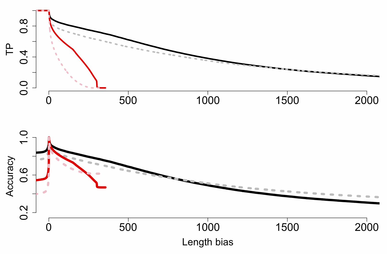
The really key thing here is that MinION reads are beating MiSeq ones at most length difference (bias) thresholds greater than ~5-10bp, right up to 300bp (the MiSeq inserts top out at this length, of course). This is important because while here we’re matching orthogonal ID cases (A. lyrata against A. thaliana, and vice versa), in a practical application we might have a third species without a reference but two possible matches, and while some loci will be closer to the first, others could match the second. So while a threshold of 1bp might technically be the best (TP rate of ~90% and close to 100% accuracy), we may want to raise the threshold to a much higher value (>50bp) and accept lower TP rates to get a better confidence.

Result 3: Species ID does not need complete genomes for reference databases, and even works with a handful of MinION reads.

One very obvious and sensible criticism of our early drafts of this was that the reference genomes we used to build BLASTN databases with are largely completely assembled. While there’s been some handwringing recently about the structural variation of these plant genomes at population level, most people accept that a high proportion of the informative sequences in these genomes are now well determined.

For most people, in most places, this will not be the case; for instance, there’s ~300,000-400,000 plant species described, but only ~180-250 public genomes. Most of those are of the fairly-low-coverage HTS WGS variety as well, so are pretty bittily assembled. Quite often these come from first-year baselining experiments in the ‘get some DNA and run it through the MiSeq then SOAP or Abyss’ mould, with N50 values in the low ‘000s.

So to test the effect of this, we artificially digested the reference genomes a few thousand times to simulate N50 values from about 100 (virtually unassembled) up to 10^6 (essentially complete), shown here in Fig 3a for N50 values from 10^0 up to 10^4, with accuracy scores calculated for a range of cutoff values:
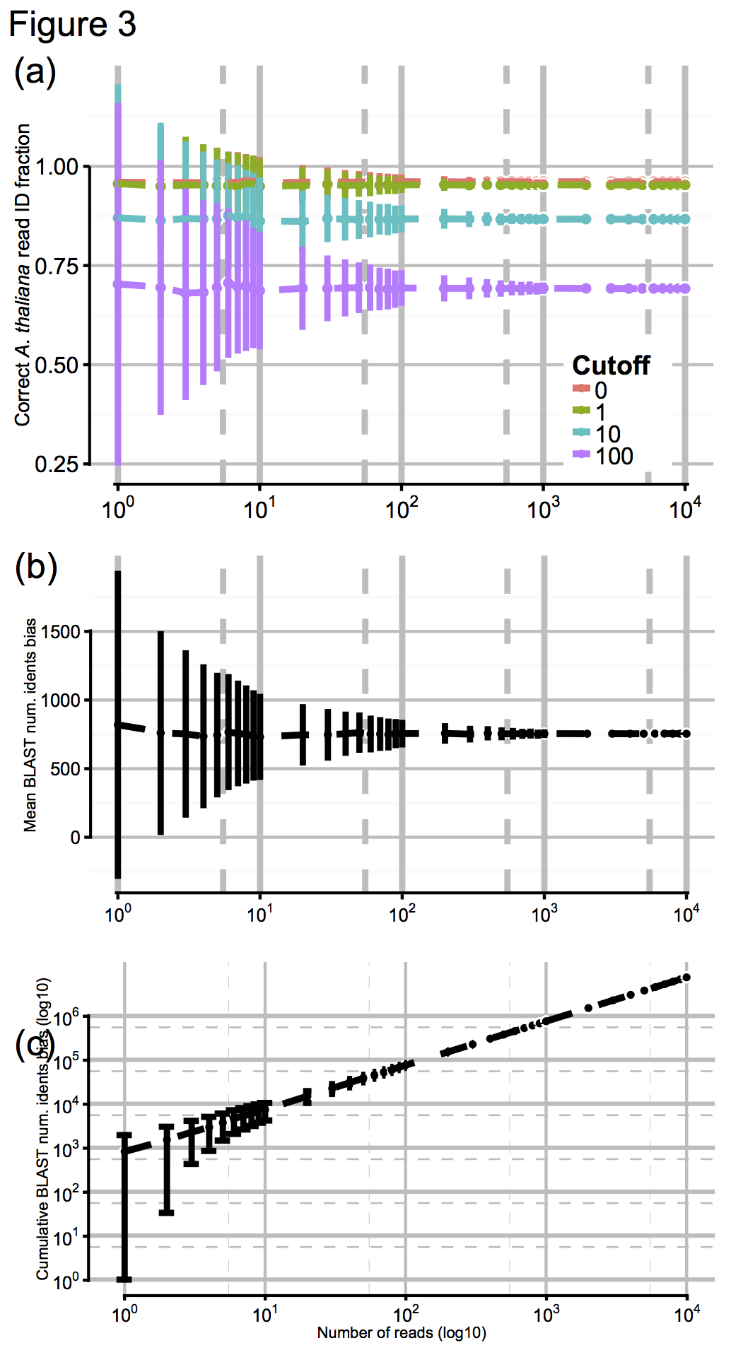
fig_3

These results were pretty promising, so finally we asked ourselves: OK, we had tens of thousands of MinION reads to make our ID with, generated over a day or so: but how few reads we would need to have a stab at a correct ID? Again, we jacknifed our dataset to find out, shown above in Figs 3b and 3c. Promisingly, you can see that by about 10^2-10^3 reads (in practice, an hour or less) the confidence intervals on our ID score barely budge. So, after an hour of sequencing, you’re likely to get as good an answer as you can get. One. Hour…!!!

Result 4: Field-sequenced WGS MinION long-reads substantially improve downstream genomics with low-coverage HTS data.

When planning the fieldwork we hadn’t really known what we’d get, in terms of read length, quality, or yield: this was a prototype kit that not many people had played with yet, let alone taken into the field. But about the time we were writing this up we found out about various genome assemblers optimised (supposedly) for ONT reads, chiefly Canu and hybrid-SPAdes. We decided to give it a whirl.. the results are pretty amazing!

Data MiSeq only MiSeq + MinION
Assembler Abyss hybridSPAdes
Illumina reads, 300bp paired-end 8,033,488 8,033,488
Illumina data (yield) 2,418 Mbp 2,418 Mbp
MinION reads, R7.3 + R9 kits,

N50 ~ 4,410bp

96,845
MinION data (yield) 240 Mbp
Approx. coverage 19.49x 19.49x + 2.01x
Assembly key statistics:
# contigs 24,999 10,644
Longest contig 90 Kbp 414 Kbp
N50 contiguity 7,853 bp 48,730 bp
Fraction of reference genome (%) 82 88
Errors, per 100 kbp:                           #N’s 1.7 5.4
# mismatches 518 588
# indels 120 130
Largest alignment 76,935 bp 264,039 bp
CEGMA gene completeness estimate:
# genes 219 of 248 245 of 248
% genes 88% 99%

Result 5: Individual MinION reads can be directly, individually annotated for coding loci with no assembly required.

By now everyone was getting a bit sick of me going on about MinION reads, but there was one final hunch I wanted to test: If reads are about the same length as nuclear coding loci (~5000-50,000bp), does that mean we can annotate individual reads to pull out coding sequences, and use them to build phylogenies? SNAP was a great tool for this, not least because it’s trained on A. thaliana gene models already.

I want to be absolutely clear here, as sometimes people seem to miss this: I’m not talking about assembling reads before annotation as usual. I’m not even talking about assembling them in real-time, then annotating. I mean, each time a read finishes basecalling, immediately try and annotate that single read, and only that single read, to try and get a coding sequence. 

In other words, how quickly can we turn a tube of DNA, into a folder of sequence reads, into alignments of coding loci? The answer is, ‘bloody quickly’:
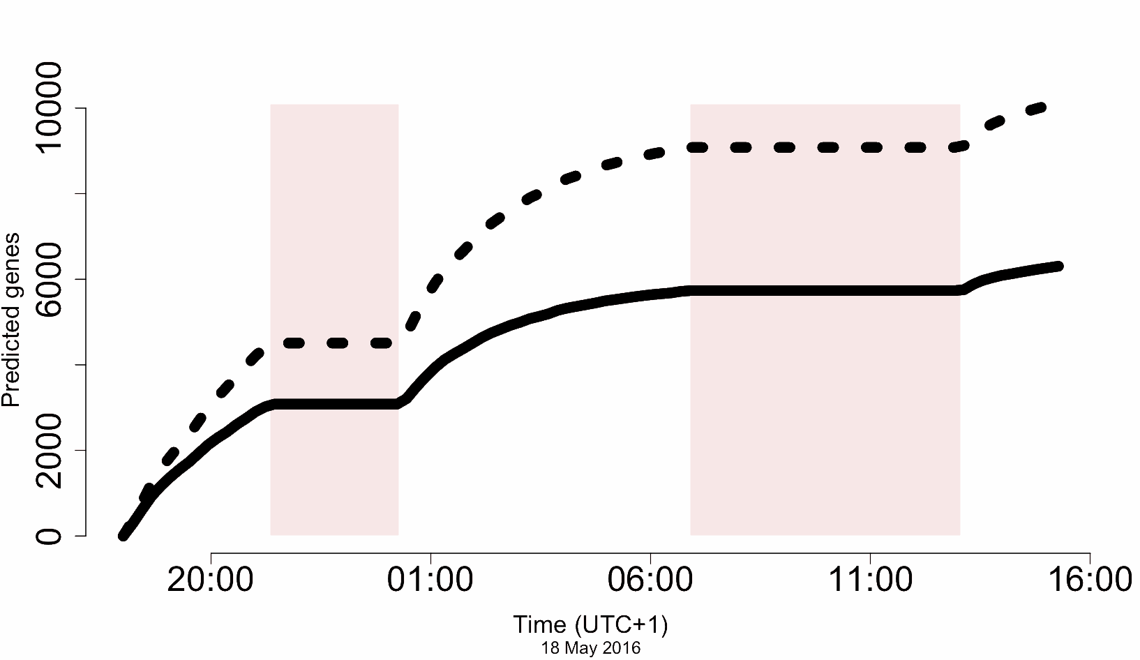
Figure_2e_genes

The dashed line shows ‘all gene models’. The solid line shows unique CDS. The axis is the number of predicted CDS and yes, those are thousands – recall that the total number of CDS for A. thaliana is only about 23,000. The axis is, well, actual sequencing time (!)*

Now, not all of these are complete genes, and error rate means distinguishing paralogs robustly in a real case (e.g. completely novel genome) would be tricky, but on the other hand, this was a completely unoptimised pipeline, really just hacked together over a couple of weeks. There’s a lot of scope to improve this…

*These are the read timestamps, but it wasn’t a live run. I actually ran the analysis back in the lab afterwards, as my code was too buggy on the fieldwork day and I just lost my shit. But the CPU demands aren’t high – I can and have run this live subsequently.


Result 6: Predicted coding loci from individual MinION reads can be aligned to orthologous sequences, and multilocus phylogeny inferred in real-time.

I build trees. I build trees. I build trees for a living. Did you seriously think, that having got as far as spitting out thousands of novel coding loci per day in field-based sequencing, I wasn’t going to try some real-time, field-based, multilocus phylogenomic inference?
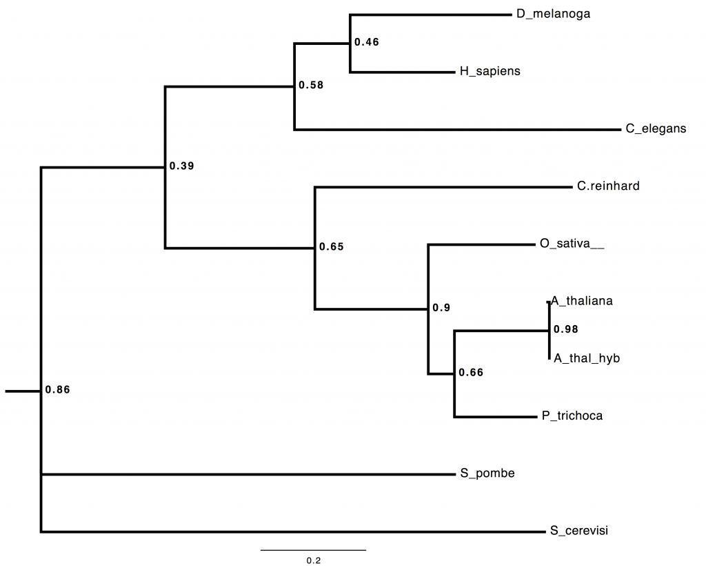
Figure_X_tree_hybridSPAdes

Here’s a *BEAST tree from 53 loci, all of the A. thaliana ones coming from directly-annotated, field-sequenced reads. Seriously 😉

Summary

As you’ve gathered by now, I’m enormously happy with this research. I think this paper is easily a bigger contribution to general science than our 2013 molecular convergence one because, if we’re honest, it’s an interesting but niche phenomenon, whereas literally everyone who uses or categorises any kind of biological material can benefit from this paper.

I’m indebted to my colleagues, Alex S. T. Papadopulos, Dion Devey, Andrew Helmstetter and Tim Wilkinson, and our funders, the Kew Foundation. We didn’t invent the MinION – that took hundreds of incredibly clever people at Oxford Nanopore years and millions of pounds of investment to do – but in this study we’ve managed to show all of the really transformative aspects of this technology working in the field, in real-time. There is no technical reason, at all why we shouldn’t all expect that within a decade, all of the analyses we currently run on DNA data in labs can run in the field, within minutes of collecting biological samples. And that really is something.

What is ‘real-time’ phylogenomics?

Over the past few years I’ve been developing research, which I collectively refer to as ‘real-time phylogenomics’ – and this is the name of our mini-site for MinION-based rapid identification-by-sequencing. Since our paper on this will hopefully be published soon, it’s probably worth defining what I hope this term denotes now, what it does not – and ultimately where I hope this research is going.

‘Phylogenomics’ is simple enough, and Jonathan Eisen at UC Davis has been a fantastic advocate of the concept. Essentially, phylogenomics is scaled-up molecular systematics, with datasets (usually derived from a genome annotation and/or transcriptome) comprising many coding loci rather than a few genes. ‘Many’ in this case usually means hundreds, or thousands, so we’re typically looking at primarily nuclear genes, although organelles’ genomes may often be incorporated, since they’re usually far easier to reliably assemble and annotate. The aim is, basically to average phylogenetic signal over many loci by combining gene trees (or an analogous approach) to try and obtain phylogenies with higher confidence (single- or few-locus approaches, including barcodes no matter how judiciously chosen, capable of producing incorrect trees with high confidence). The process is intensive, since genomes must be sequenced and then assembled to a sufficient standard to be reasonably certain of identifying orthologous loci. This isn’t the only use of the term (which also refers to phylogenies produced from whole-genome metagenomics) but the most straightforward and common one as far as eukaryote genomics is concerned, and certainly the one uppermost in my mind.

However the results are often confusing, or at least more complex than we might hope: instead of a single phylogeny with high support from all loci, and robust to the model used, we often find a high proportion of gene trees (10-30%, perhaps) agree with each other, but not the modal (most common, e.g. majority rule consensus) tree topology. For instance among 2, 326 loci in our 2013 paper on phylogenomics of the major bat families, we found that position of a particular group of echolocators – which had been hotly debated for decades, based on morphological and single-locus approaches – showed such a pattern (sometimes supporting the traditional grouping of Microchiroptera + Megachiroptera, but over 60% of loci supporting the newer Yangochiroptera + Yinpterochiroptera system. This can be for a variety of reasons, some biological and some methodological. The point is that we have a sufficiently detailed picture to let us chose between competing phylogenetic hypothesis with both statistical confidence and intuition based on comparison.

These techniques have been on the horizon for a while (certainly since at least 2000) and gathered pace over the last decade with improvements in computing, informatics, and especially next-generation sequencing. The other half of this equation, ‘real-time’ sequencing, has emerged much more recently and centres, obviously, on the MinION sequencer. Most work using this so far has focused either on the very impressive potential long-read data offers for genomic analyses, particularly assembly, or rapid ID of samples e.g. the Quick/Loman Zika and Ebola monitoring studies; and our own work.

So what, exactly, do we hope to achieve with phylogenomic-type analyses using real-time MinION data, and why?

Well, firstly, our work so far has shown that the existing pipeline (sample -> transport -> sequence-> assemble genome-> annotate genes-> align loci-> build trees) has lots of room for speedups, and we’re fairly confident that the inevitable tradeoff with accuracy when you omit or simplify certain steps (laboratory-standard sequencing, assembly) is at least compensated for by the volume of data alone. Recall that a ‘normal’ phylogenomic tree similar to our bat one might take two or more postdocs/students a year to generate from biological samples, often longer. A process taking a week instead would let you generate something like 50 more analyses in a year! The most obvious application for this is just accelerating existing research, but the potential for transforming fieldwork and citizen science is considerable. This is because you can build trees that inform species relationships, even if the species in question isn’t known. In other words a phylogenome can both reliably identify an unknown sample, and also identify if it is a new species.

More excitingly, I think we need to have a deeper look at how we both construct and analyse evolutionary models. Life on earth can be accurately and fully described best by a network, not a bifurcating tree, but this applies to loci as well as single genes. In other words, there is a single network that connects every locus in every living thing. Phylogenetic trees are only a bifurcating projection of this, while single- or multi-locus networks only comprise a part.

We’ve hitherto ignored this fact, largely because (a) trees are often a good approximation, especially in the case of eukaryote nuclear genes, and (b) the data and computation requirements a ‘network-of-life’ analysis implies are formidable. However, cracks are beginning to appear, in both faces. Firstly, many loci are subject to real biological phenomena (horizontal gene transfer, selection leading to adaptive convergence, etc) which give erroneous trees as discussed above. Meanwhile prokaryotic and viral inference is rarely even this straightforward. Secondly, expanding computing power, algorithmic complexity, and sequencing capacity (imagine just 1,000 high schools across the world, regularly using a MinION for class projects…) mean the question for us today really isn’t ‘how do we get data’, but ‘how ambitious do we want to be with it?’

Since my PhD but especially since 2012, I’ve been developing this theme. Ultimately I think the answer lies in the continuous analysis of public phylogenomic data. Imagine multiple distributed but linked analyses, continuously running to infer parts of the network of life, updating their model asynchronously both as new data flood in, and by exchanging information with each other. This is really what we mean by real-time phylogenomics – nothing less than a complete Network of Life, living in the cloud, publicly available and collaboratively and continuously inferred from real-time sequence data.

So… that’s what I plan to spend the 2020s doing, anyway.


Some aspects of BLASTing long-read data

Quick note to explain some of the differences we’ve observed working with long-read data (MinION, PacBio) for sample ID via BLAST. I’ll publish a proper paper on this, but for now:

  • Long reads aren’t just a bit longer than Illumina data, but two, three, four or possibly even five orders of magnitude longer (up to 10^6 already, vs 10^2). This is mathematically obvious, but extremely important…
  • … the massive length means lots of the yield is in comparatively few reads. This makes yield stats based on numbers of reads positively useless for comparison with NGS. Also…
  • Any given long read contains significantly more information than a short one does. Most obviously the genomics facilities of the world have focused on their potential for improving genome assembly contiguity and repeat spanning (as well as using synteny to spot rearrangements etc) but we’ve also shown (Parker et al, submitted) that whole coding loci can be directly recovered from single reads and used in phylogenomics without assembly and annotation. This makes sense (a ~kb long read can easily span a whole gene, also ~kb in scale) but it certainly wasn’t initially obvious, and given error rates, etc, it’s surprising it actually works.
  • Sample ID using BLAST actually works very differently. In particular, the normal ‘rubbish in, rubbish out’ rule is inverted. In other words, nanopore reads (for the time being) may be long, but inevitably contain errors. However, this length means that assuming BLAST database sequences are approximately as long/contiguous, Nanopore queries tend to either match database targets correctly, with very long alignments (hundreds/thousands of identities), or not at all.

This last point is the most important. What it means is that, for a read, interpreting the match is simple – you’ll either have a very long alignment to a target, or you won’t. Even when a read has regions of identity to more than one species, the correct read has a much longer cumulative alignment length overall for the correct one. This is the main result of our paper.

The second implication is that, as it has been put to me, for nanopore reads to be any good for an ID, you have to have a genomic database. While this is true in the narrow sense, our current work (and again, this is partly in our paper, and partly in preparation) shows that in fact all that matters is for the length distribution in the reference database to be similar to the query nanopore one. In particular, we’ve demonstrated that a rapid nanopore sequencing run, with no assembly, can itself serve as a perfectly good reference for future sample ID. This has important implications for sample ID but as I said, more on that later 😉

More MinION – the ‘1D rapid’ prep

My last MinION post described our first experiments with this really cool new technology. I mentioned then that their standard library prep was fairly involved, and we heard that the manufacturers, Oxford Nanopore, were working on a faster, simpler library prep. We got in touch and managed to get an early prototype of this kit for developers*, so we thought we’d try it out. So our** experiments had three aims:

  • Try out this new rapid kit
  • Try out different extraction methods, to see how they worked with the kit
  • See if we could sequence some fairly damaged DNA with the kit

This is a lot of combinations to perform over a few days on one sequencing platform! Our experience from the last run gave us hope we could manage it all (we did, but with a lot of headaches over disk space – it turns out one drawback of being able to run multiple concurrent sequencing runs is hard-drive meltdown, unless you’re organised from the start – oops). In fact, to keep track of all the reads we added an ‘index’ function to the Poretools package. I really recommend you use this if you’re planning your own work.

We had eight samples to sequence, a 15-year-old dried fungarium specimen of Armillaria ostoye (likely to be poor quality DNA; extracted by Bryn Dentinger with a custom technique); some fresh Silene latifolia (Qiagen-extracted, which we’d used successfully with the previous, ‘2D’ library prep); and six arbitarily-selected plant samples, both monocots and dicots, extracted by boiling with Chelex beads (more about them at the end).

IMG_4555

First we prepared normal ‘2D’ libraries from the Silene and Armillaria. These performed as expected from our December experiments, even the Armillaria giving decent numbers and lengths of reads (though not as many as we hoped, with some indication of worse Q-scores. We put this down to nicks in the fungarium DNA, and moved on to the 1D preps while the sequencer was still running.

The ‘1D’ in the rapid kit (vs ‘2D’ in the normal kit) refers to how many DNA strands are sequenced; in the 2D version, both forward and reverse-complement strands are sequenced. This is slower to prepare (extra adapters etc to link the two strands for sequencing) and also runs through the MinION more slowly (twice as much DNA, plus a hairpin moment) but is roughly twice as accurate, since each base is read twice. The 1D kit, on the other hand, results in single-stranded fragments, meaning we could expect lower accuracy traded off for higher speed. And the rapid kit really was fast – starting from purified extracted DNA, we added all the necessary adapters for sequencing in well under 15mins, ready to sequence.

lenQuals
The sequencing itself (for both the Armillaria and the Silene) went spectacularly well. Remember, this is unsheared genomic DNA, and imagine our surprise when we started to see 25, then 50, then 100, then 150kb reads come off the sequencer – many mapping straight away to reference genomes! It turns out that the size distribution of the 1D prep is much more long-tailed than the 2D/g-TUBE one. In fact, whereas the the 2D library looks like a normal-ish gamma, the 1D reads are more like an inverse exponential – lots of short stuff and then a very long tail with some mega-whopper reads in. Reads so long, in fact, that mapping them the same way as Illumina short-read data would be a bit bonkers…

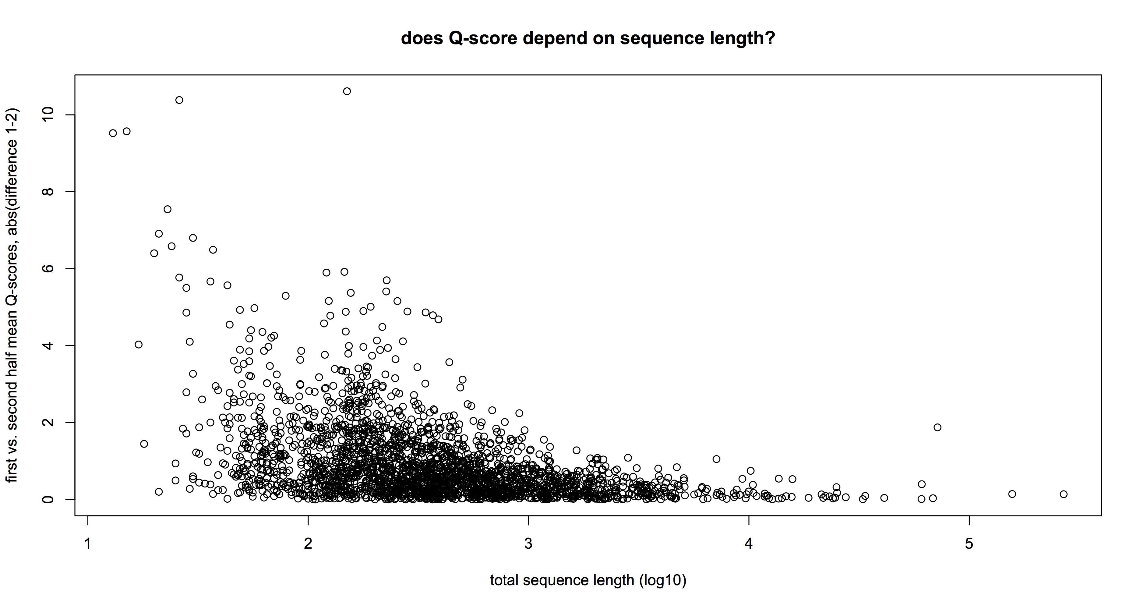
As for accuracy, well, the Q-scores are definitely lower in the 1D prep; around half the 2D as we expected. On the other hand, they were still matching reference databases via BLAST/BLAT/BWA quite happily – so if your application was ID, who cares? Equally, combining mega-long 1D reads with more shorter but accurate reads could be a good way to close gaps in a de novo genome sequencing project. One technical point – there is definitely a lot more relative variation in the Q-scores for short (<1000bp) reads than for longer ones: the plot above shows the absolute difference in mean Q-scores in (first – vs – second) halves of a subset of 2,300 1D reads. You can see that below 1kb, Q-score variation exceeds 4 (bad news when mean is about there) while longer reads have no such effect (quick T-test confirms this).

So in short, the 1D prep is great if you just want to get some DNA on your screen ASAP, and/or long reads to boot. In fact, if you came up with a way to size-select all the short gubbins out before sequencing, you’d have one mega-cool sequencing protocol! What about the last bit of our test – seeing if a quick and dirty extraction could work, too? The results were… mixed-to-poor. Gel electrophoresis and Qubit both suggested the extracted DNA was pretty poor quality/concentration, and if we didn’t believe them, the gloopy, aromatic, multicoloured liquid in the tubes supplied direct evidence to our eyes. So rather than test those samples first (and risk damaging a perfectly good flowcell early on in the experiment), we held them back until the end when only a handful of pores were left. In this condition it’s hard to say whether they worked, or not: the 50 or so reads we got over an hour or two from fewer than 10 pores is a decent haul, and some of them had some matches to congenerics in BLAST, but we didn’t really give them a full enough test to be sure.

Either way, we’ll be playing around with this more in the months to come, so watch. This. Space…


*Edit: Oxford Nanopore have recently announced that the rapid kit will be out in April for general purchase.

**Again working, for better or worse, with fellow bio-beardyman Dr. Alex Papadopulos. Hi Alex! This work funded by a Royal Botanic Gardens, Kew Pilot Study Grant.

Copying LOADS of files from a folder of LOADS *AND* LOADS more in OSX

Quick one this, as it’s a tricky problem I keep having to Google/SO. So I’m posting here for others but mainly myself too!

Here’s the situation: you have a folder (with, ooh, let’s say 140,000 separate MinION reads, for instance…) which contains a subset of files you want to move or copy somewhere else. Normally, you’d do something simple like a wildcarded ‘cp’ command, e.g.:

1
host:joeparker$ cp dir/*files_I_want* some/other_dir

Unfortunately, if the list of files matched by that wildcard is sufficiently long (more than a few thousand), you’ll get an error like this:

1
-bash: /bin/cp: Argument list too long

In other words, you’re going to have to be more clever. Using the GUI/Finder usually isn’t an option either at this point, as the directory size will likely defeat Finder, too. The solution is pretty simple but takes a bit of tweaking to work in OSX (full credit to posts here and here that got me started).

Basically, we’re going to use the ‘find’ command to locate the files we want, then pass each one in turn as an argument to ‘cp’ using ‘find -exec’. This is a bit slower overall than doing the equivalent as our original wildcarded command but since that won’t work we’ll have to lump it! The command* is:

1
find dir -name *files_I_want* -maxdepth 1 -exec cp {} some/other_dir \;</p>

Simple, eh? Enjoy 🙂

*NB, In this command:

  • dir is the filesystem path to start the search; ‘find’ will recursively traverse the directory tree including and below this folder;
  • -name *glob* gives the files to match;
  • -maxdepth is how deep to recurse (e.g. 1 = ‘don’t recurse’);
  • cp is the command we’re executing on each found file (could be mv etc);
  • {} is the pipe argument standing for the found file;
  • some/other_dir is the destination argument to the command invoked by -exec

Messing about with the MinION

IMG_4543Molecular phylogenetics – uncovering the history of evolution using signals in organisms’ genetic sequences – is a powerful science, the latest expression of the human desire to understand our common origins. But for all its achievements, I’d always felt something was, well lacking from my science. This week we’ve been experimenting with the MinION for the first time, and now I know what that is: immediacy. I’ll return to this theme later to explain how exciting this realisation is, but first we better ask:

What is a MinION?

NGS nerds know about this already, of course, but for the rest of us: The MinION (minh-aye-on) is a USB-connected device marketed by a UK company, Oxford Nanopore, as ‘a portable real-time biological analyser’. Yes – that does sound a lot like a tricorder, and for good reason: just like the fictional device, it promises to make the instant identification of biological samples a reality. It does this using a radically different new way to ‘read’ DNA sequences from a liquid into a letters (‘A, C, G, T‘) on a computer screen. Essentially, individual strands of DNA are pulled through a hole (a ‘nanopore’) in an artificial membrane, like the membranes that surround every living cell. When an electric field is applied to the membrane, the individual DNA letters (actually, ‘hexamers’ – 6-letter chunks) passing through the nanopore can be directly detected as fluctuations in the field, much like a magnetic C-60 cassette tape is read by a magnetic tape head. The really important thing is that, whereas other existing DNA-reading (‘sequencing’) machines take days-to-weeks to read a sample, the MinION produces output in minutes or even seconds. It’s also (as you can see in the picture, above) a small, wait tiny device.

Real-time

This combination of fast results and small size makes the tricorder dream possible, but this is more than just a gadget. Really, having access to biological sequences at our fingertips will completely change biology and society in many ways, some of which Yaniv Erlich explored in a recent paper. In particular, molecular evolutionary biologists will soon be able to interact with their subject matter in ways that other scientists have long taken for granted. What I mean by this is that in many other empirical disciplines, researchers (and schoolkids!) are able to directly observe, or easily measure, the phenomena they study. Paleontologists dig bones. Seismologists feel earthquakes. Zoologists track lions. And so on. But until now, the world of genomic data hasn’t been directly observable. In fact reading DNA sequences is a slow, expensive pain in the arse. And in such a heavily empirical subject, I can’t help but feel this is a hindrance – we are burdened with a galaxy of baroque models to explain variations in the small number of observations we’ve made, and I’ve got a hunch more data would actually consign many of them to the dustbin.

Imagine formulating, testing, and validating or discarding genetic hypotheses as seamlessly as an ecologist might survey a new forest…

IMG_4531

Actual use

That’s the spiel, anyway. This week we actually used the MinION for the first time to sequence DNA (I’d been running some other technical tests for a couple of months, but this was our first attempt with real samples) and since it seems lots more colleagues want to ask about this device than have had a chance to use it, I thought I’d share our experiences. I say ‘we’ – work took place thanks to a Pilot Study Fund grant at the Royal Botanic Gardens, Kew, in collaboration with Dr. Alex Papadopulos (and really useful input from Drs. Andrew Helmstetter, Pepijn Kooij and Bryn Dentinger). It’s worth pointing out that although there’s a lot of hype about the device, it is still technically in a prototype/public-beta type phase, so things are changing all the time in terms of performance, etc.

IMG_4547First up, the size. The pictures don’t really do it justice… compared with existing machines (fridge-sized, often) the MinION isn’t small, it’s tiny. The thing itself, plus box and cable, would easily fit into a side pocket on any laptop bag. So the ‘portable’ bit is certainly true, as far as the platform itself is concerned. But there’s a catch – to prepare a biological sample for sequencing on the MinION, you first have to go through a fairly complicated set of lab steps. Known collectively as ‘library preparation’ (a library here meaning a test tube containing a set of DNA molecules that have been specially treated to prepare them to be sequenced), the existing lab protocol took us several hours the first time. Partly that was due to the sheer number of curious onlookers, but partly because some of the requisite steps (bead cleanups etc) just need time and concentration to get right. None of the steps is particularly complicated (I’m crap at labwork and just about followed along) but there’s quite a few, and you have to follow the steps in the protocol carefully.
Performance

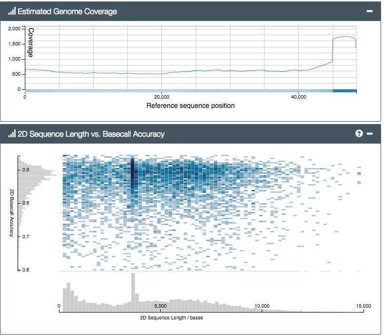
So how did the MinION do? We prepared two libraries; one from a control sample of bacteriophage lambda (a viral genome, used to check the lab steps are working) and another from Silene latifolia, a small flowering plant and one of Alex’s faves. The results were exciting. In fact they were nerve-wracking – initially we mixed up the two samples by mistake (incredible – what pros…) and were really worried when, after a few hours’ sequencing, not a single DNA read matching the lambda genome had appeared. After a lot of worrying, and restarting various analyses, including the MinION itself, we eventually realised our mistake, reloaded the MinION with the other sample and – hey presto! – lambda reads started to pour out of the software. In the end, we were able to get a 500x coverage really quickly (see reads mapped to the reference genome, below):

lambda

You can see from the top plot that we got good even coverage across the genome, while the bottom plot shows an even (ish) read length distribution, peaking around 4kb. We’d tried for a target size of 6kb (shearing using g-TUBEs), so it seems the actual output read size distribution is lower than the shearing target – you’d need to aim higher to compensate. Still, we got plenty of reads longer than 20, or even 30,000 base-pairs (bp) – from a 47kbp genome this is great, and much much much longer than typical Illumina paired-end reads of ~hundreds of bp.

Later on the next day, we decided we’d done enough to be sure the library preparation and sequencing were working well, so we switched from the lambda control to our experimental (S.latifolia) sample. Again, we got a good steady stream of reads, and some were really long, over 65,000bp. Crucially, we were able to BLAST these against NCBI and get hits against the NCBI public sequence database and get Silene hits straight back. We were also able to map them onto the Silene genome directly using BWA, even with no trimming or masking low-quality regions. Overall, we got nearly a full week’s sequencing from our flowcell, with ~24,000 reads at a mean length of ~4kb. Not bad, and we’d have got more if we hadn’t wasted the best part of the run sodding about while we troubleshot our library mix-up at the start (the number of active pores, and hence sequencing throughput, declines over time).

The bad: There is a price for these long, rapid reads. Firstly, the accuracy is definitely lower than Illumina – although the average lambda library sequencing accuracy in our first library was nearly 90%, on some of our mapped Silene reads it dropped much lower – 70% or so. This has been well documented, of course. Secondly, the *big* difference between the MinION in use and a MiSeq or HiSeq is the sheer level of involvement needed to get the best from the device – whereas both Illumina machines are essentially push-button operated, the MinION seems to respond well if you treat it kindly (reloading etc) and not if you don’t (introducing air bubbles while loading seemed to wreck some pores)

The very, very, good: Ultimately though, we came away convinced that these issues won’t matter at all in the long run. ONT have said that the library prep and accuracy are both boing improved, as are flowcell quality (prototype, remember). Most importantly the MinION isn’t really a direct competitor to the HiSeq. It’s a completely different instrument. Yes, they both read DNA sequences, but that’s where the similarity ends. The MinION is just so flexible, there’s almost an infinite variety of uses.

In particular, we were really struck that the length of the reads means simple algorithms like BLAST can get a really good match from any sample with just a few hundreds, or tens, of reads from a sample. You just don’t need millions of 150bp reads to match an unknown sample to a database with reads this long! Coupled with the fact that the software is real-time and flowcells can be stopped and started, and you have the bones of a really capable genetic identification system for all sorts of uses; disease outbreaks (in fact see this great work on Ebola using MinION); customs control of endangered species; agriculture; brewing – virtually anything, in fact, where finding out about living organisms’ identity or function is needed.

The future.

There’s absolutely no question at all: really, these devices are the future of biology. Maybe the MinION will take off (right now, the buzz couldn’t be hotter), or a competitor will find a way to do even more amazing things. It doesn’t matter how it comes about, though – the next generation of biologists really will be living in a world where, in 10, 15, 20 years, at most, the sheer ubiquity of sequencers like this will mean that most, if not all eukaryotes’ genomes will have been sequenced, and so can be easily matched against an unknown sample. If that sounds fantastic, consider that the cumulative sequencing output of the entire world in 1988 amounted to a little over 100,000 sequences, a yield equivalent to a single good MinION run. And while most people in 1988 thought that, since the human genome might take 30 or 40 years to sequence, there was little point in even starting, a few others looked around at the new technology, its potential, and drew a different conclusion. The rest is history…